Why measure weight?
Steady Scale is built on a simple premise: awareness gives you choices. Regularly recording your weight helps you see meaningful changes while they are still small, whether that's recognizing progress sooner or noticing an unintended drift early enough to respond.
Frequent self-weighing has consistently been associated with greater weight loss, less regain, and better long-term maintenance.1,2,3 These studies cannot establish causation, but they suggest that regular measurement helps people notice gradual changes before they become large ones.
The same principle applies after reaching a goal. Among people who have kept weight off, consistent self-monitoring is associated with lasting success, while letting the habit lapse is associated with regain.4 A slow drift is difficult to notice from one measurement to the next; a trend makes it visible while it is still small.
The psychological side has been studied too. A large meta-analysis found that, for most adults, self-weighing is not associated with disordered eating or poorer body image, although some groups, particularly younger people, showed small negative associations with well-being.5
These findings shaped the design. Rather than encouraging more weighing through reminders or streaks, the app tries to make each measurement more informative. The goal is not to react to every fluctuation, but to understand meaningful changes when they appear. Its language stays body-neutral, never treating a single number as a judgment.
The problem: separating signal from noise
Your weight changes from one morning to the next for many reasons besides body fat. Water balance, glycogen stores, sodium, meal timing, and gut contents can all move the scale substantially over a day or two.6
Every weigh-in therefore contains two things: the long-term direction your weight is moving, and short-term fluctuations that say little about body composition. The challenge is separating them.
Our solution
Steady Scale estimates your trend in two steps.
First, every reading recorded during a day is averaged into a single daily value. Extra measurements do not add noise; they sharpen the estimate of that day's weight.
Second, the app fits a ridge regression through the previous fourteen days of daily averages. The fitted value at the present day is your current trend.
That is the entire trend model.
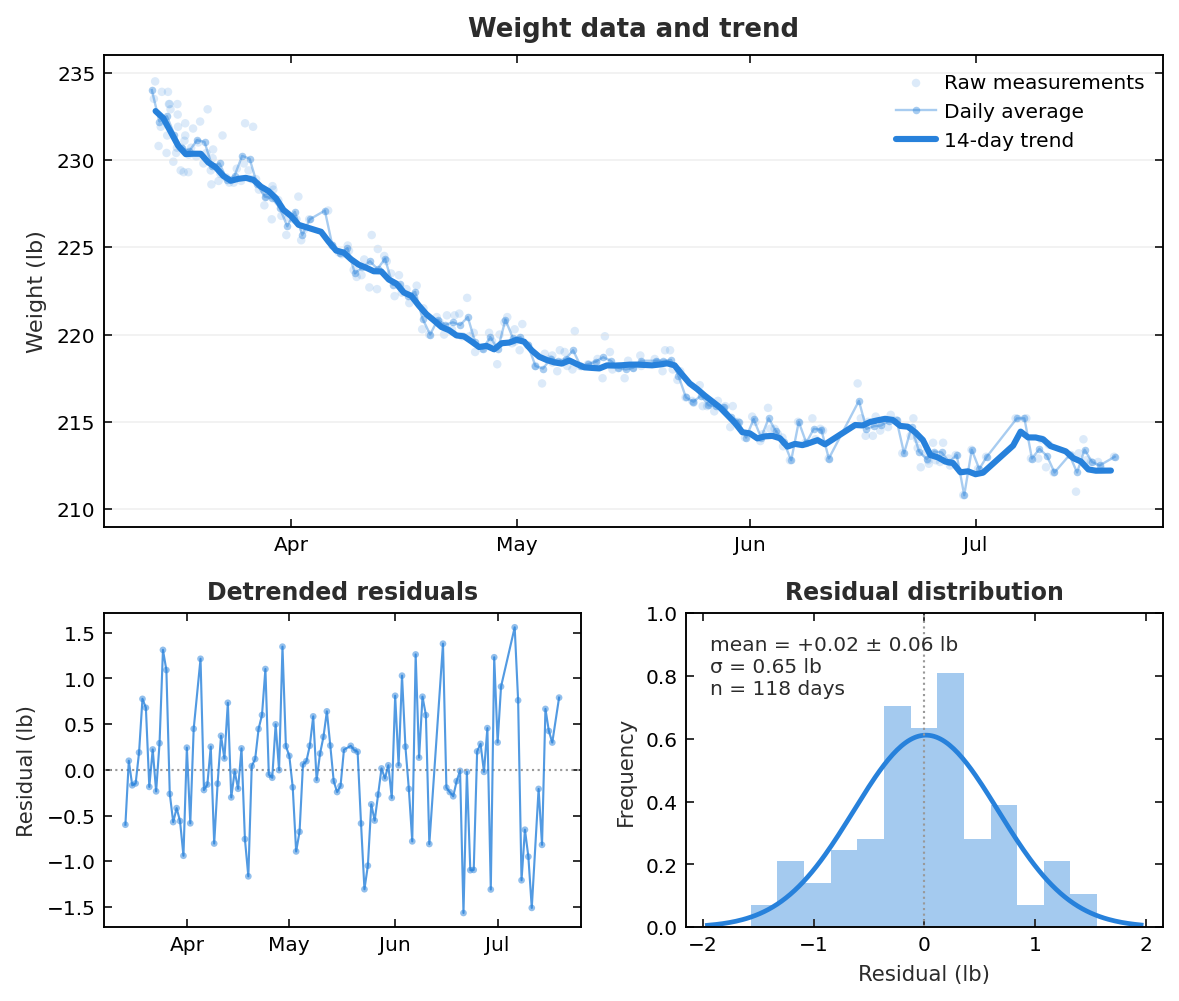
Figure 1 shows the model applied to four months of real weigh-ins. It also shows the residuals, the difference between each daily average and the fitted trend. Centered on zero, the residuals behave like random measurement noise rather than a missed pattern, suggesting the trend captures the systematic movement without introducing bias.
Choosing the trend model
A model that explains yesterday perfectly is not necessarily the model that predicts tomorrow best. So we treated the design as an optimization problem: compare combinations of model type and window length, and keep the one that forecasts best.
We compared eight candidate models, including moving averages, ordinary and weighted regressions, exponential smoothing, and more flexible curve fits, across a range of window lengths. Each combination was repeatedly fitted to its trailing window, asked to predict the days ahead, and scored on its errors, on real data and on simulated scenarios with plateaus, rate changes, and gaps in logging.
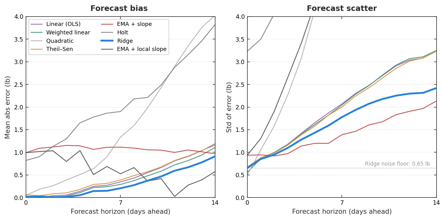
The result illustrates a classic trap. The models with the smallest fitting errors, the ones that followed every local fluctuation, produced the largest forecasting errors. The best-performing combination was not the one that reproduced the past most faithfully. It was a fourteen-day ridge regression.
It may not draw the smoothest line, but it consistently produced the most accurate forecasts with the least overall bias.
Why ridge regression?
Every trend model makes the same trade-off. A highly flexible model follows every fluctuation: it fits yesterday's measurements extremely well, but produces unstable forecasts because it mistakes random variation for real change. An overly smooth model has the opposite problem: it ignores the noise, but reacts slowly when your weight genuinely begins to change.
The challenge is finding the right balance between these extremes. Ridge regression strikes that balance by penalizing large swings in slope, accepting a small increase in fitting error in exchange for a more stable estimate of the underlying direction.7
The model can be written compactly. The trend at day t is a straight line,
whose intercept and slope are chosen to minimise the ridge objective:
Here y represents the daily averages from the previous fourteen days and x the day they were measured. The final term, λβ₁², is what distinguishes ridge regression from ordinary least squares. It discourages steep slopes that are only weakly supported by the data, reducing overreaction to short-term fluctuations. The app uses λ = 1 with time measured in days.
The result is intentionally conservative. The trend is not designed to react to every measurement. It is designed to react when the evidence supports a genuine change.
Why fourteen days?
Window length is a similar compromise. Short windows respond quickly, but much of what they respond to is noise. Long windows are steadier, but increasingly describe where your weight was rather than where it is now: a trailing window takes roughly its own length to fully reflect a genuine change.
In the same test, forecast accuracy improved rapidly up to about ten days, then showed diminishing returns. Longer windows became slightly steadier, but increasingly lagged behind genuine changes because they relied on older measurements. Fourteen days was the shortest window that captured nearly all of the improvement in forecast accuracy while remaining responsive to genuine changes.
That is the window Steady Scale uses.
How accurate is it?
Understanding the accuracy of the model helps put its estimates into context.
Because the forecast predicts the trend rather than an individual weigh-in, we evaluated it against the trend itself. We repeatedly asked the model where it expected the trend to be several days later, then compared each prediction with the trend calculated after those measurements became available. We tested the model on both real and simulated data covering weight loss, weight gain, maintenance, and datasets with plateaus and different day-to-day variability. Typical forecasting error was 0.2 to 0.5 lb one day ahead, 0.5 to 1.2 lb three days ahead, and 1.1 to 2.8 lb seven days ahead.
A seven-day forecast is best thought of as a preview based on your current trajectory, not a prediction set in stone. A lot can change over the course of a week. As new measurements arrive, the forecast updates and its uncertainty narrows. When projecting just one day into the future, the underlying trend can typically be estimated within a few tenths of a pound. This is significant considering that normal day-to-day fluctuations in body weight are often much larger.
These results also define the limits of the model. The forecast estimates where your trend is heading, not what the scale will read tomorrow morning. And it cannot anticipate changes that have not happened yet. If your eating, activity, or routine changes, the estimate changes with it. A forecast that never moved would look more certain, but it would be less honest.
The same uncertainty applies to long-term projections. Rather than presenting a single confident goal date, the app shows a range that widens over time, reflecting the growing uncertainty of longer forecasts.